Abstract

Shawn Carlson's 1985 study on astrology, published in Nature, has been highly influential in critiques of astrology as a scientifically valid phenomenon. However, the closure drawn on astrology in the study, based on the lack of statistical significance in the linear regression analysis of astrologers' performance, remains questionable. In this article, we revisit Carlson's study, focusing on Figure 2 and the linear regression. Applying modern, algorithmic influence-testing using Cook Distances and DFBETAS, we examine potential outliers and reformulate the best fit line, yielding relevant rankings of 1-8, comprising 93.8% of data. The resulting regression relation (y = 0.507 + 0.0954 x) has an ANOVA p-value for the slope term of 0.0113, indicating the astrologers' actions do have a statistically significant effect. R-squared for this model is 0.684. Our findings suggest that Carlson's conclusion might not adequately consider modern statistical techniques, even as they were available to him, and further quantitative analysis of astrology may still be relevant today.


Introduction
​
In 1985, a recent Bachelor of Science graduate, Shawn Carlson, published in the premier science magazine (then or now) -- Nature -- a study of astrology!

​It “was prepared as an account of work sponsored by the United States Government” and was declared “… a perfectly convincing and lasting demonstration” by the journal’s editor. [1]

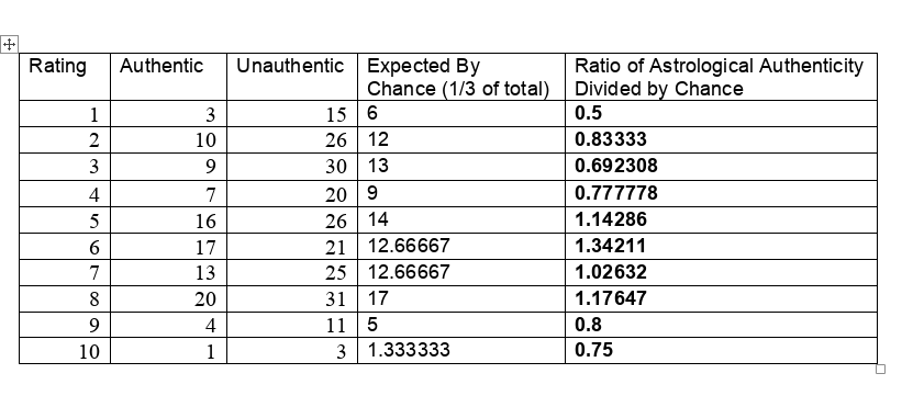
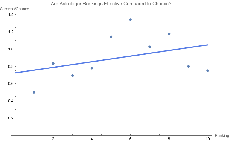
To say that the paper was and is influential would be a disservice. It is the single most effective critique of astrology in recent times. [1]

Arguably the paper served the interests of debunkers and assuaged renascent throes of concern about astrology in the Euro-American general and scientific culture. Some forty years later, Carlson’s test of astrology also still  influences the position of many astrologers who contend that astrology is beyond quantitative analysis and is better understood as an art than a science. [1].

While Carlson was working on the astrology study, a new statistician, R. Dennis Cook was just beginning his publication career. Cook’s contributions have proven to be prescient, protean, and vast. [2, 3]

Whether you are a skeptic, debunker, or even a fan of astrology, it is important to know that Carlson’s limited study now must be said to be highly constrained by Cook’s much more far-ranging and massive work, work used in scientific crucibles of the highest capacity and resting easy on the transformative bonfires of time.

A Problem

There are many problems in construction, presentation, and conclusion with the Carlson study. [1] Here we will be focusing on Figure 2, the regression line.
​
First, let’s consider the data. Consistent with the publication standards of the time, Carlson did not release the original data. However, from Figure 3 in his paper the original tabular data may be surmised. [1] They are the following.

​The chosen astrologers endeavored to match charts to their owners. In a sort of double-blind fashion, the astrologers were given one true chart and two false options. They were asked to rate each match from one (least certain) to ten (most certain).
​
When the last column of data is graphed with its best fit line, a dismal picture emerges.

​The best fit line is y = 0.724701 +0.03262x with an ANOVA p-value of fit for the slope of the line being 0.276045. In other words, one can not claim that the slope (a measure of effect) is different from that for a flat line which has a slope of zero. 

That is to say, no statistical significance is found in the astrologers' actions compared to chance.

Carlson relies heavily on the lack of significance in this type of regression relation in his conclusions.

Is this the end of the story? Astrology is dead?

Not at all.

As others have brought up, there are major, legitimate, and co-existing concerns with the methodology of the study as a whole, such as:

• the entropic travels of the experimental design
• Likert-type issues
• manipulation of sample size that balloons the chance of a false negative (and a negative is what was found here)
• the fact that the absence of proof is not proof of absence
• and there are actually many more. [1] [8]

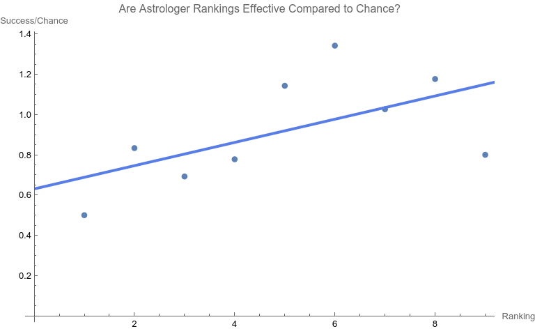
I will focus on the particular linear regression above.

The Solution

Returning to one of the preeminent statisticians of our era, Cook innovated in many ways, and a preeminent one is the use of “Cook Distances” to identify highly influential points. [4]

“.... Cook's distance and DFFITS are conceptually identical.... Previously when assessing a dataset before running a linear regression, the possibility of outliers would be assessed using histograms and scatterplots [Ed: as did Carlson]. Both methods of assessing data points were subjective and there was little way of knowing how much leverage each potential outlier had on the results data. This led to a variety of quantitative measures, including DFFIT, DFBETA....” [4]

Influential points are not bad in themselves, but they do need to be checked for being an undue outlier. The rational and consistent way to do this in recent years is through Cook Distances and DFBETAS. [5, 6, 7]

An iterative, one-case deletion algorithm is appropriate for our one-variable linear regression. [9] The approach as a whole is not too complicated in practice:

1. Compute the linear regression relation (as shown above).
2. Check each point (and there are only at most 10 here) for Cook Distances that are higher than the conventional cut-off of 0.5. [7]
3. For each such point, compute the DFBETAS for effect on the slope of the linear regression which again is the measure of effect size that we are interested in.
4. If the absolute value of DFBETAS is higher than the conventional cutoff of two divided by the square root of n, that point is determined to be an outlier and should be removed from consideration.[6]
5. Return to step one until all points are below outlier cut-offs.

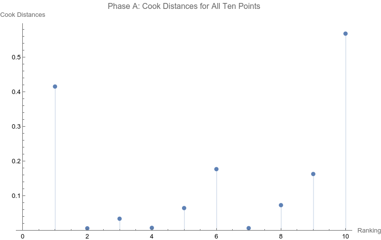
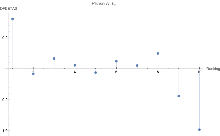
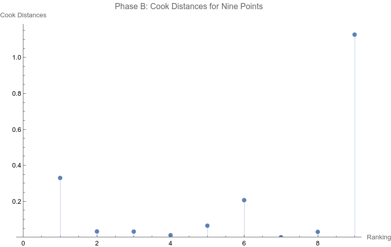
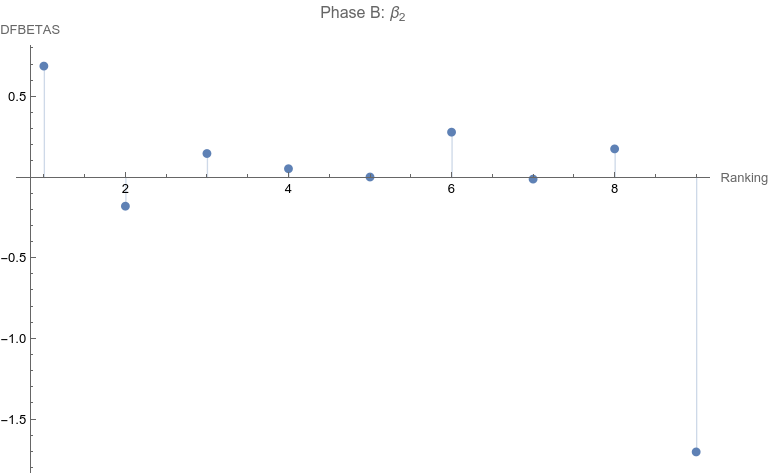
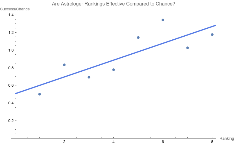
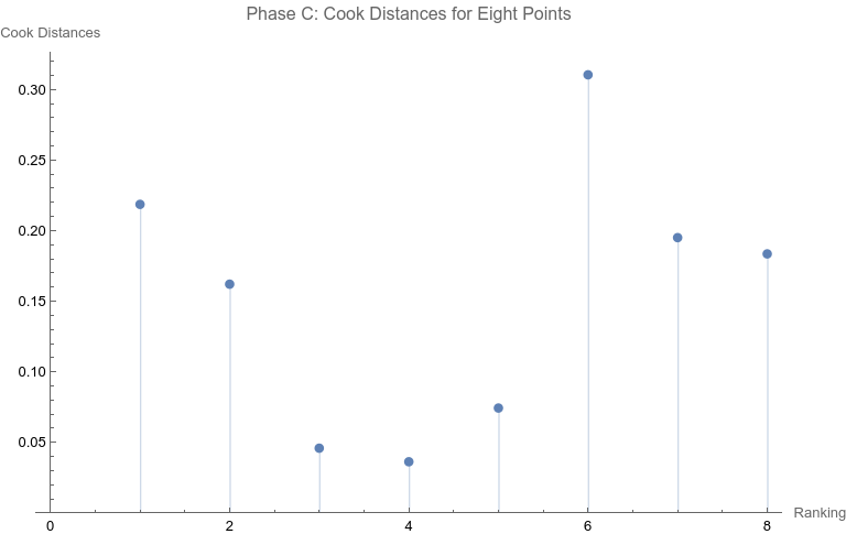
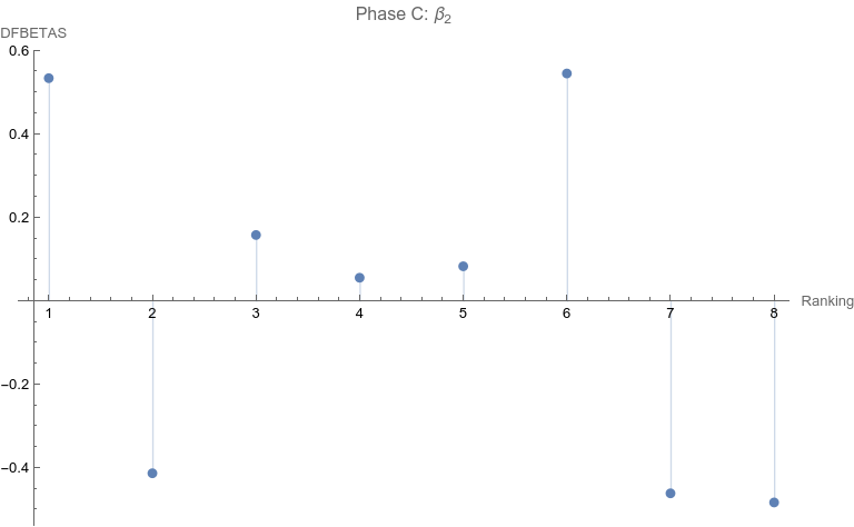
Note that none of the steps in these tests are based on p-values. Let’s apply the set of computations to the data above.

Phase A: All 10 points are considered
​
1. The regression relation is depicted and described above.
2. 

​The ranking of 10 is the only point that has a Cook Distance greater than the cut-off of 0.5. It is a candidate for consideration for DFBETAS for the slope. 
​
3. 

​​4. The cutoff for n = 10 here is 2 divided by the square root of 10 or 0.632456. The point identified from step 2 that corresponds to a ranking of 10 has an absolute value that far exceeds that cut-off. It is thus a strong candidate as an outlier influence and should be removed.
 
Phase B: Rankings only of 1 through 9 are considered
​
1.  The best fit linear regression is depicted.

The regression relation is y = 0.632761 + 0.0576959 x with an ANOVA p-value for fit for the slope term of 0.0950004. 
​
The fit looks better already, but we have to follow the steps of the algorithm.

​2. 

Here there is a clear outlier point at ranking of 9 whose Cook Distance far exceeds 0.5. It is a candidate for DFBETAS computation.
​
3.  

​4. The cutoff for n = 9 here is 2 divided by the square root of 9 or 0.66667. The point identified from step 2 that corresponds to a ranking of 9 has an absolute value that far exceeds that cut-off. It is thus a strong candidate as an outlier influence and should be removed.

Phase C: Rankings only of 1 through 8 are considered

​1 . 

The regression relation is y = 0.507038 + 0.0954128 x with an ANOVA p-value for fit for the slope term of 0.0112811.

The fit looks way better behaved than how we started, but we still have to follow the steps of the algorithm.

2.

​3. None of the Cook Distances are above the conventional cut-off of 0.5. We may conclude the algorithm.
​
4. For completion’s sake, the DFBETAS for rankings 1 through 8 are depicted below. None of the |DFBETAS| for the slope term are above the conventional cut-off of 2 divided by the square root of 8 or 0.70711.

​Conclusion

We have thus found through rigorous, modern influence-testing that the best fit line is more truly:

y = 0.507038 + 0.0954128 x

with an ANOVA p-value for fit for the slope term of 0.0112811. 

​The effect size may be said to be 0.0954128 per unit increase of rank. R-squared for the entirety of this final model is 0.684298 which is another measure of effect.

As a bonus to applying the algorithm in this case, the cost of removing outlier influence is not dear. Only 6.17%, a small number of chart matches out of the total of 308, needs to be removed (n = 4  for the ranking of ten and n = 15 for the ranking of nine). Those two rankings also happen to be the smallest groups of the ten.

Moreover, the final regression relation suggests that astrologers' sense of authenticity of the chart compared to chance is only greater than one when the ranking is at five or above. This is exactly what one would hope.

The removal of the 9th and 10th rankings is not because they are inconvenient but because standard contemporary diagnostic algorithms for point sensitivity in a linear regression require us to remove them.

After all, "failure to conduct post model fitting diagnostics for variance components can lead to erroneous conclusions about the fitted curve." [9]

​We have to gather that yes, there is effect in the astrologers’ actions, and this positive assessment is not hampered by an undue chance of it being a false positive, since the p-value of 0.0112811 is less than the conventional one-sided alpha of 0.05.

Nature should retract the article.

Sites Cited
​
[1] http://www.astrology-research.net/researchlibrary/U_Turn_in_Carson_Astrology_Test.pdf

[2] http://users.stat.umn.edu/~rdcook/CookPage/Bio.pdf

[3] http://users.stat.umn.edu/~rdcook/CookPage/cookcv.pdf

[4] https://en.wikipedia.org/wiki/DFFITS

[5] https://www.bookdown.org/rwnahhas/RMPH/mlr-influence.html

[6] https://data.library.virginia.edu/detecting-influential-points-in-regression-with-dfbetas/

​[7] https://online.stat.psu.edu/stat462/node/173/

[8] https://independent.academia.edu/KennethMcRitchie

[9] https://escholarship.org/content/qt54h3s321/qt54h3s321_noSplash_5481a8a81db5affca388b35aab6964d4.pdf

Abstract

The belief in a correspondence between the planetary positions at the time of a world event and those at a similar event at another time is ancient and still claimed today (Tarnas, 2006). Using a database of 6770 dates of world events after January 1, 1600, AD from Wolfram Research, the short descriptions that accompany each date are quantified using 1536 long embeddings from OpenAI. Embeddings, a gift from machine learning, are a precise way to measure similarities between text. They were used here to quantify similarities in short descriptions without dates of pairs in 6770 world events post-1600 AD as found in a provided database. There are 22913065 unique such possible pairs. The zodiacal placements of the charts were also calculated for either the actual date at midnight of the event or the same but
using the start date for a multi-day event. Only Sun, Moon, Mercury, Venus, Mars, Jupiter, Saturn, Uranus, Neptune, Pluto, North Lunar Node, and South Lunar Node Tropical degree placements from zero to 360 degrees were computed. Finding the mean of the Cosines of the differences between planetary placements for two events offers a neat and novel way of measuring similarities between these zodiacal placements for the two events. These metrics for textual similarities and chart similarities when plotted against each other suggest non-monotonic dependence with effect size between the chart extrema being 0.380. The upper p-value for independence between the two metrics is less than 0.0001 as computed by Hoeffding’s dependence measure. The conservative Monte Carlo approach to estimating the upper value of this p-value was necessary due to physical computation constraints. Thus, likelihood for the alternative to independence, namely dependence, between event textual similarities and event chart similarities is shown. A classifier for an event date being war-like or peace-like as decided by similarity of the embeddings for the event’s full description to the embeddings for the words “war” and “peace” respectively was successful as built on event zodiacal placements only.


Introduction 
World events are often used in astrology studies. Accurate places, dates, and times are typically known even when they are not precise, allowing for a bridge between astrological placements and interpretation of social, cultural, and personal significations.  
 
Studies of the correlation between celestial positions and world events are ancient. Over six centuries during the first millennium BCE, scholars in Mesopotamia recorded nightly celestial positions and terrestrial events onto clay diaries known as menologies. So, while they might log a full moon aligned with Venus in the constellation of Taurus, they also recorded mundane events such as the price of grain, the water levels in the Euphrates River or an earthquake (Sachs 1988) (Rochberg-Halton 1991). 
 
Rarely however do these studies include enough events to achieve statistical significance for the interpretations drawn.  
 
This practice has continued into modern times. Cultural historian, Richard Tarnas documents historical evidence to support a correspondence between mundane events and astrological alignments in his book, Cosmos and Psyche (2006). 
 
The problem with verifying these claimed correlations statistically is that it is hard to measure such a diverse range of events objectively and consistently. Here I use a textual description of 6838 historical events in relation to astrological placements at the time of the event. 
 
Across many millions of pairs of events, is the size of difference in textual descriptions (which contain words loaded with social, cultural, and personal significance) related to magnitude of difference in astrological charts for the two events? 
 
I will be exploring quantitative equivalencies for most of the concepts within this question and then use appropriate mathematics to answer it.

Materials and Methods 

Full code is available, including for the generation of event data (Oshop, 2023). 

Almost all of the calculations in this study were performed through the professional mathematics software, Mathematica, which offers many tools. One of those is a database of 7818 historical events (Wolfram Research, 2012). 
 
Included in the database for each event is a one sentence text-description (e.g., "Apollo 8 Returns to Earth") and the start date (e.g., December 27, 1968). Source information and metadata is not available for this database beyond assurances that it is continually being updated (Wolfram Research, 2022) (Wolfram Research, 2022). Unfortunately, this database is anglophone-centric, but alternatives are hard to come by as simple and easily accessible event databases are surprisingly rare. 
 
The data was pared down to 6838 events from 7818 by excluding dates prior to 1600 AD and all events whose start date was January 1. The first was to reduce uncertainty resulting from the switch from the Julian to the Gregorian calendar that was phased in globally from 1582 AD. The latter was to obviate a problem with the database, wherein uncertain dates for events were sometimes listed as January 1 of the year.  

All numbers and other specifying qualifiers were also algorithmically removed from the database event descriptions. This was to avoid an artificial connection. For example, “The Battle of 1812” could be unrelated to another event that has the year 1812 in its description. (So, “The Battle of 1812” is reduced to “battle”.) Care was also taken to ensure that there were no duplicates in the event database. 

Finally, removing these qualifiers in the chart descriptions to make them unspecific sometimes removed all the words in the description. Such empty event descriptions were removed from consideration, further limiting the number of events to 6770.  

The removal process was considered necessary to remove most artefacts of association through excessive adjectives. So, for example, “earthquake" was the desired distillate and not full descriptions of earthquakes which may have been chained together in a region in 1912. 

Table 1 shows the difference between the hands-off, automated distillates and original event descriptions from a random selection. Note that contemporary embeddings in general are robust enough to know when to treat names in the distillates as capitalized. For specific methods of the distilling algorithm, see the code. (Oshop, 2023)

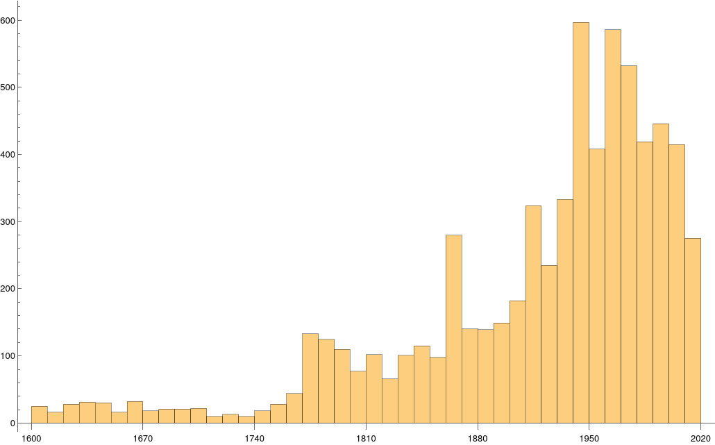
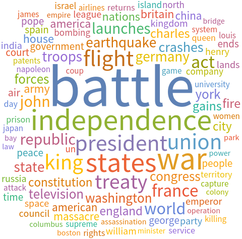
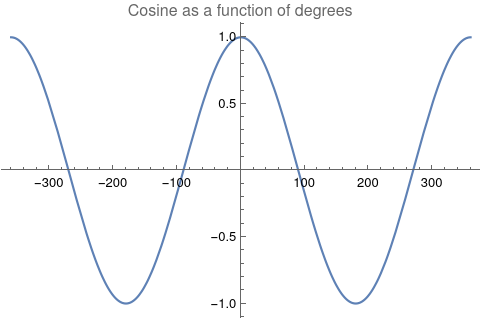
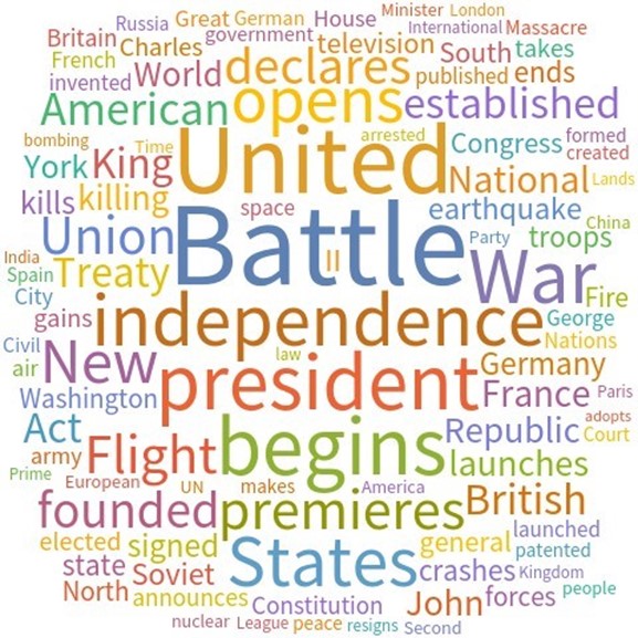
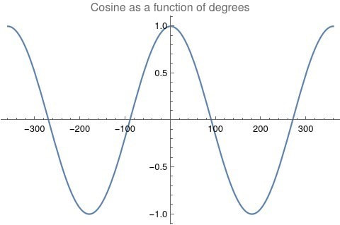
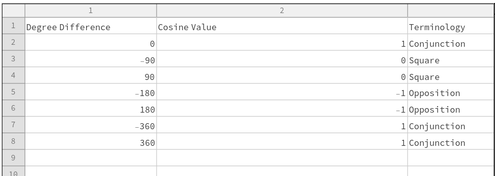
A timeline histogram of the resulting 6770 events follows in Figure 1. 

 
In Figure 2 is a word cloud of the most frequently used words in the 6770 event descriptions. 

Measuring Textual Description Similarities 
Allowing for high precision in quantitatively measuring qualitative texts, embeddings were introduced in 2003 in a paper that states that they “associate with each word in the vocabulary a distributed word feature vector … The feature vector represents different aspects of the word: each word is associated with a point in a vector space. The number of features … is much smaller than the size of the vocabulary” (Bengio, et al., 2003) (Aylien.com, 2022). 
 
These embeddings embody a literal “geometry of meaning” (Gärdenfors, 2017). To share an example from computer science literature, subtracting the embedding numbers for “man” from those for “king” and then adding those for “woman”, one gets the numbers that closely align with “queen” (MIT Technology Review, 2015). So, king - man + woman = queen. 
 
The calculator for embeddings used for this study was developed by OpenAI, was released in 2022, and uses the "text-embedding-ada-002" model. It results in a vector, a list, that is 1536 numbers long for each event’s deconstructed description. Each of the 1536 numbers in the vector is critical to fully describing the textual quality of the event description but in quantitative terms. 

Going from two 1536-featured vectors for each event pair to a single number is done by measuring the cosine distance between each pair’s event embeddings (Google Research, 2018). In general, as similarity between two vectors increases, cosine distance decreases.

Measuring Chart Similarities 

The celestial positions are measured in geocentric ecliptic longitude. While this is the same metric as the Tropical Zodiac, the values are expressed between 0° and 360° from the Vernal Point or 0° Tropical Aries. For each event there are separate degrees for Sun, Moon, Mercury, Venus, Mars, Jupiter, Saturn, Uranus, Neptune, Pluto, North Lunar Node, and South Lunar Node, thus creating a 12-number-long vector for each. Reduction to a simple number was made by taking the average of the twelve cosines of the twelve angle distances for each pair. 

Comparing the 12-digit vectors for these zodiacal placements could be done by dot product, but that would miss some key features of astrology charts. We consider charts to be highly similar or conjunct when their degree differences, i.e., the results of their degrees’ subtractions, are either close to zero or close to 360 degrees or -360 degrees. Nicely enough, there is a trigonometric function that behaves exactly this way: the cosine. The simple plot of it follows, wherein you can see that the blue line has maxima at 0 degrees, 360 degrees, and -360 degrees. 

Moreover, there are other qualities of the cosine curve that preserve information from astrology. Oppositions at +/- 180 degrees yield a cosine of -1, and +/-90-degree squares yield a value of zero. These parallel the astrological interpretations wherein squares suggest no similarity, and oppositions do show similarity but of an opposite polarity as conjunctions. Degrees in between the extrema have cosine values that are appropriately in between as well. 

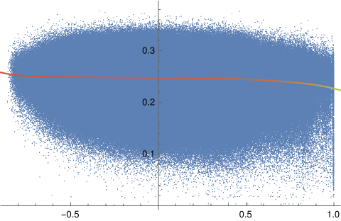
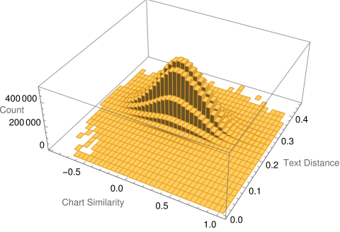
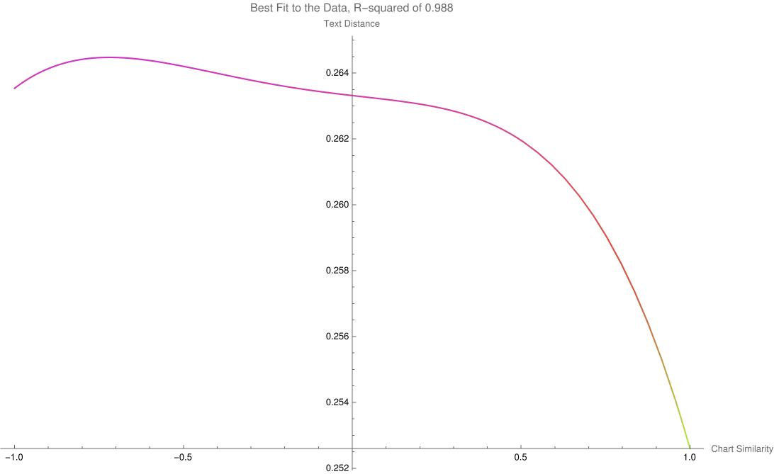
There exists a consistent bridge between astrological terminology and cosine value of degree differences between two events. 

Thus, for each of the two events in an event pair, the twelve placements of the second one was subtracted from those of the first one. Applying cosine to each of the twelve differences and then doing a simple average gives a single-number result that is a straightforward summary for the chart similarities of the 12 astronomy features.

Measuring the Relationship Between the Texts and the Planetary Positions 

Next is the assignment of detecting dependence. Note that this is different than correlation. 

For example, a quartic is a function of the order of x raised to the fourth power. The resulting graph shows for each x one f(x), but it is not so that each f(x) only corresponds to one x. Parabolas, hyperbolas, and certain trigonometric functions such as cosine depicted above behave similarly. 

Thus, one can say for these that f(x) is indeed a function of x, but not in a monotonic fashion. The idea of monotonic dependence is also known as correlation, but for these special non-monotonic functions, we need to consider tests for dependence and not correlation. 

In short: 

For dependency: determine that a variable has a value that depends on the value of another variable. 

For correlation: the relationship between variables is linear and is considered as correlation. That is, as one similarity increases the other uniformly increases or decreases too. 

This paper’s study answers a question not about correlation but about the more sophisticated situation of dependence. 

To do the answering, a tool that can compute not just linear dependence (i.e., correlation) but also non-linear dependence, namely Hoeffding’s D (for dependence) measure, was selected. 

Each Hoeffding D measure test was found to take about 16 seconds to compute for 100,000 event pairs, 22 minutes for 1,000,000 event pairs, and an unknown amount for the full event pairs that number over 25 million. The latter is unknown because the computation was aborted after six days. (The computer that was used is running Linux on an AMD 3950x CPU with 64 GB DDR4 RAM.) 

Thus, a Monte Carlo approach was needed to estimate the upper-bound “p-hat” of the actual full p-value for independence. The approach consists of breaking up the problem into computing the p-value 10000 separate times for randomized sets that number 100000 pairs each. 

The equation for this conservative upper bound is simply (r + 1) divided by (n + 1), where r is the number of runs that yield a test-statistic above that which is desired (here corresponding to a p-value of alpha 0.05) and n is the number of separate times the randomization is run (here equal to 10000). 

All that is needed is r. 

Results

In the Monte Carlo simulation, r = 0, yielding a p-hat upper value for p of (0+1) divided by (10000+1) which is less than 0.0001. 

To make it simpler to see the relationship between chart similarities to their embedding distances, here is the scatterplot of measurements in blue with their best fit line. 

The three-dimensional histogram edition is shown in Figure 5 wherein a subtle shift from higher counts in the upper left dropping to the lower right is seen. As the charts become more similar, description distances become smaller, and description similarities become greater. 

The general trend is subtle but clearer in Figure 6, wherein the nonlinear, algorithmically determined, best fit curve is shown, 

y=0.263316−0.00117471x+0.000483782x^2−0.00429352x^3−0.00573389x^4=0

which has an adjusted R-squared of 0.988 for fit and ANOVA p-values for coefficients that are far less than 0.0001. The relationship between the two variables is not monotonic which explains why dependence and not correlation is more proper.

The effect size (Cohen’s D) in text distance when the chart similarity is one, compared to when it is minus one, is 0.380.

A functional relationship between historical event text descriptions and historical event celestial placements is thus established.

Successful classifier test

To further test the utility of this relationship, each event description's similarity to the single-word texts of “war” and “peace” was found through cosine distance of their embeddings. Where the similarity to “war” was higher, the event’s astronomy chart set was associated with the classification of W, else the event astronomy was classified as P. Cloneable data is accessible. (Oshop, 2023)

After a random 80%-20% split of data into a training set and test set, the best performing model (determined via cross-validation) was a boot-strap decision forest model. The top field importances for the model are Saturn (4.52%), Sun (4.64%), Uranus (5.12%), Pluto (10.98%), and Neptune (54.25%). Access to the interactable and cloneable model is also available (Oshop, 2023)

Testing the model on the 20% test set yielded success in classifying P 95.5% of the time and W 22.9% of the time, outperforming both random choice and modal choice in recall, accuracy, precision, f-measure, and phi-coefficient.

More extensive, interactable, and detailed results are available.  (Oshop, 2023)

Conclusions

A function for similarity applied to historical event descriptions is shown to be a function of chart similarity with a p-value for independence that is far lower than 0.001. 

Calculating similarities between the celestial degrees on any arbitrary day and those of the nearest events in the database (even when full descriptions are not known) based on that astrology is nearly trivial. The demonstrated loose similarity of charts to these events’ descriptions may allow for some mundane event prediction. This study brings us closer to that potential future. 

As a demonstration of the general utility of the astronomy chart of an event holding predictive power, a classification of event astronomies into war or peace was found to have more utility than either a random 50-50 choice or choosing the more common peace classification each time. One may apply this classifier to future astronomies.  

As a preliminary result, it does indeed seem there is a time for war and a time for peace, as well as astronomical ways to understand a moment’s relationship to historical events that have gone before.  

All material for replication is included in references. (Oshop, 2023). 

 
References 
Aylien.com (2022) An overview of word embeddings and their connection to distributional semantic models, https://aylien.com/blog/overview-word-embeddings-history-word2vec-cbow-glove 

Bengio Y., Ducharme R., Vincent P., and Jauvin C. (2003) A Neural Probabilistic Language Model, Journal of Machine Learning Research, 1137–1155, 
https://www.jmlr.org/papers/volume3/bengio03a/bengio03a.pdf 

Gärdenfors P., The Geometry of Meaning (2017) MIT Press https://mitpress.mit.edu/books/geometry-meaning 

Google Research Inc. (2002) Measuring Similarity from Embeddings, 
https://developers.google.com/machine-learning/clustering/similarity/measuring-similarity 
 
MIT Technology Review (2015) King - Man + Woman = Queen: The Marvelous Mathematics of Computational Linguistics, https://www.technologyreview.com/2015/09/17/166211/king-man-woman-queen-the-marvelous-mathematics-of-computational-linguistics/ 

Oshop R. (2023) Is Text Similarity of Events Related to Chart Similarity? https://www.wolframcloud.com/obj/renay.oshop/Published/EventsComparisonCode.nb  

Oshop R. (2023) BigML Cloneable Data https://bigml.com/shared/dataset/y5gOLoQb1y9Ikkhgi9st8ASDXXd 

Oshop R. (2023) BigML Cloneable OptiML https://bigml.com/shared/ensemble/6AitpIkSL1tYyAEi1WCYMsZqDMi 
 
Oshop R. (2023) BigML Test Set Results https://bigml.com/shared/evaluation/9HxONbPHG3iVER1FxfgRzHMKZVS   

Rochberg-Halton, Francesca (1991) The Babylonian Astronomical Diaries. Journal of the American Oriental Society Vol. 111, No. 2 (Apr. - Jun.), pp.323-332  

Sachs, A.J. & Hunger, H. (1988) Astronomical Diaries and Related Texts from Babylonia, Austrian Academy of Sciences, Vienna.  

Tarnas, Richard (2006) Cosmos and Psyche: Intimations of a New World View, New York: Viking  

Wolfram Research (2012) EventData, https://reference.wolfram.com/language/ref/EventData.html  

Wolfram Research (2022), Frequently Asked Questions, https://www.wolframalpha.com/faqs/  

Wolfram Research (2022), Wolfram Knowledgebase, https://www.wolfram.com/knowledgebase/ 

Early narrative explaining results as of May 13, 2022 (presentation for OPA Research):

The slide set:

Whiteboard explainer video:

Download the Powerpoint slide set which includes the video:

The below is automated daily data cultivation with automated daily aggregate analysis in Wolfram Mathematica:

Daily Data [click to download csv file]

To download or use a copy of the code immediately above, click on the three lines in the bottom left and then choose "make your own copy" or "download". There is a free time-limited version of Mathematica that you can use with the download, or making your own copy will open up an online version of the software that you can use for free.

Finally, use the below to cultivate the daily asteroid namesake article counts:

Python code for cultivation of daily data

import requests
from bs4 import BeautifulSoup
import pandas as pd
from datetime import date
from datetime import timedelta
#import numpy as np


#dataset containing 1200 names
df = pd.read_csv('names to search Fiverr A.csv')

#creating a list of all 1200 names
all_names = df['NAME'].values
#input_date = '2022-02-16'

input_date0 = date.today()-timedelta(days =1)#gives yesterday date
input_date = input_date0.isoformat()
#print(input_date)


#input_date = input('Enter the date in format yyyy-mm-dd example 2022-02-03:  ')

#Generating Urls from given list of names
def get_url(name):
    url_template = 'https://news.google.com/search?q={}'
    url = url_template.format(name)
    return url



#Scraping news title and date
def get_news(article,name):
    #title = article.h3.text
    title_date = article.div.div.time.get('datetime').split('T')[0]
#    print(title_date)
    if title_date == input_date:
        all_data = (title_date,name)
    return all_data


#Main function to run all code

main_list = []
def Main_task():
    for news_name in all_names:
        records = []
        count = 0
        url = get_url(news_name)
        response = requests.get(url)
        soup = BeautifulSoup(response.text,'html.parser')
        articles = soup.find_all('article','redacted')

        for article in articles:
            try:
                all_data = get_news(article,news_name)
                records.append(all_data)

            except:
                continue
        count = len(records)
#        print("---")
        main_list.append((news_name,count))

Main_task()
mynamedata = pd.DataFrame(main_list,columns= ['NAMES',input_date])
mynamedata.to_csv(input_date+'.csv')

Abstract

Embeddings, a way to measure similarities between texts, are a recent gift of machine learning. They were used here to quantify similarities in very short descriptions without dates of pairs in 7153 world events post-1600 AD as found in a provided database. There are 25,579,128 unique such possible pairs. The zodiacal placements of the charts were also calculated for either the actual date at midnight of the event or the same but using the start date for a multi-day event. Only Sun, Moon, Mercury, Venus, Mars, Jupiter, Saturn, Uranus, Neptune, Pluto, North Lunar Node, and South Lunar Node Tropical degree placements from zero to 360 degrees were computed. Adding up the Cosines of the differences between planetary placements for two events offers a neat and novel way of measuring similarities between these zodiacal placements for the two events. Thus, I have metrics for textual similarities and chart similarities. The imagery of these metrics plotted against each other suggests non-monotonic dependence. This study answers a precise question: what is the p-value for independence between the two metrics? The upper p-value for independence is less than 0.01 as computed by Hoeffding’s dependence measure. The conservative Monte Carlo approach to estimating the upper value of this p-value was necessary due to physical computation constraints. Thus, likelihood for the alternative to independence, namely dependence, between event textual similarities and event chart similarities is established. A separate Hoeffding's dependence measure for each celestial feature is calculated for the special case of event distances to the word "Battle". A Monte Carlo simulation shows that these separate Hoeffding's D measures are mostly extremely unlikely given the distributions of celestial degrees in the data. Wolfram language code and data are included.

Introduction

World events are often used in astrology studies. Accurate place, date, and time are typically known even when they are not precise, allowing for a bridge between astrological placements and interpretation of social, cultural, and personal significations.

Rarely however do these studies include enough events to achieve statistical significance for the interpretations drawn.

Instead, I posit a more general and more foundational hypothesis: across many millions of pairs of events, is the magnitude of difference in textual descriptions (which contain words loaded with social, cultural, and personal significance) related to magnitude of difference in astrological charts for the two events?

I will be exploring quantitative equivalencies for most of the concepts within this question and then use appropriate mathematics to answer it.

Materials and Methods

All of the calculations in this study were performed through the professional mathematics software, Mathematica, which offers many tools, one of which is a database of 7818 historical events.[1]

Included in the database is a one sentence text-description (eg "Apollo 8 Returns to Earth") and start date (eg Dec 27 1968). Source information and metadata is not available for this database beyond assurances that it is continually being updated.[2][3]

Unfortunately, this database is largely anglophone-centric, but alternatives are hard to come by as more general event databases are surprisingly hard to access.

The first step to cultivating the data was the choice to include only events that took place at and after the year 1600 AD. The reasoning is that there was a calendrical revolution with the introduction of the Gregorian system around year 1582 with delays in adoption in some cultures that took many years.

This restriction of date pares the 7818 events down to 7153 events.

A timeline plot of the events follows.

Next, I removed all numbers in the database event descriptions, because I do not want to connect similarity between eg “The Battle of 1812” and another event that may have the year 1812 in its description. (So, “The Battle of 1812” is reduced to “The Battle of”.) To not do this would allow de facto some correspondence of text description and chart placements which I want to avoid. Care was also taken to assure that there were no duplicates in the event database.

A word cloud of the most common words in the resultant event descriptions follows.

For pair construction, 7153 options are available for the first event and 7152 are available for the second event. Multiplying these and dividing by two to erase repetition yields 25,579,128 possible unique pairs. The following analysis is applied to each pair.

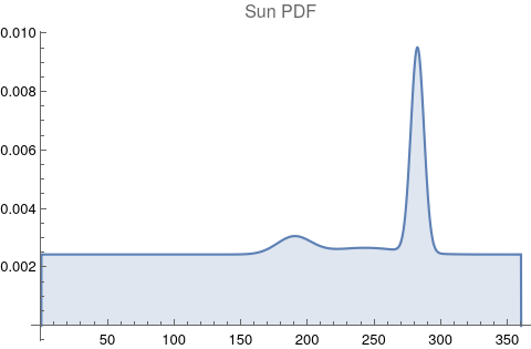
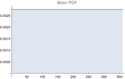
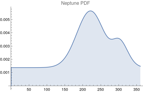
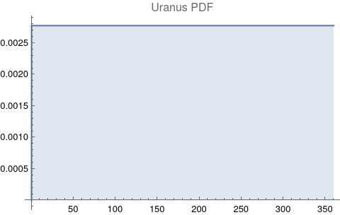
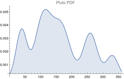
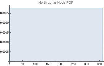
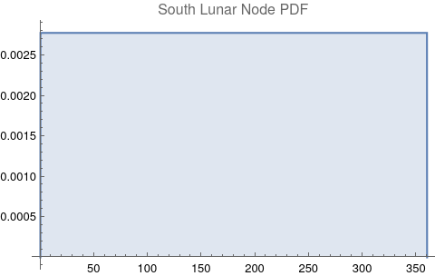
The questions for each pair are:
a. “How exactly similar are their textual descriptions?”,
b. “How exactly similar are their planetary placements?”, and
c. “Do these two similarities correspond to each other?”

For a. only since early 2000’s AD is there a way to more precisely measure this trait of qualitative texts. Embeddings were introduced in 2003 in a paper that states that they “associate with each word in the vocabulary a distributed word feature vector … The feature vector represents different aspects of the word: each word is associated with a point in a vector space. The number of features … is much smaller than the size of the vocabulary”.[4][5]

These embeddings embody a literal “geometry of meaning”.[6] To share an example from popular computer science literature, subtracting the embedding numbers for "man" from those for "king" and then adding those for "woman", one gets the numbers that closely align with "queen".[7] So, king - man + woman = queen.

The particular calculator for embeddings used for this study was developed by Google Research, Inc., was released in 2018, and is called Bidirectional Encoder Representations from Transformers (BERT).[8] It results in a vector, a list, that is 768 numbers long for each event description. The similarity metric between two event descriptions is simply the dot product of their 768-number-long vectors.[9] Decapitalization did not affect the calculations.

Next is the assignment b. to compare the Tropical zodiac placements for the dates of each event pair and have a similarity measure. These geocentric ecliptic longitude placements are values between 0 degrees and 360 degrees and are also the degree placements used in Tropical astrology. For each event there are separate degrees for Sun, Moon, Mercury, Venus, Mars, Jupiter, Saturn, Uranus, Neptune, Pluto, North Lunar Node, and South Lunar Node, thus creating a 12-number-long vector for each.

Descriptive plots for the probability distribution function (PDF) of each celestial feature as a function of degrees follow.

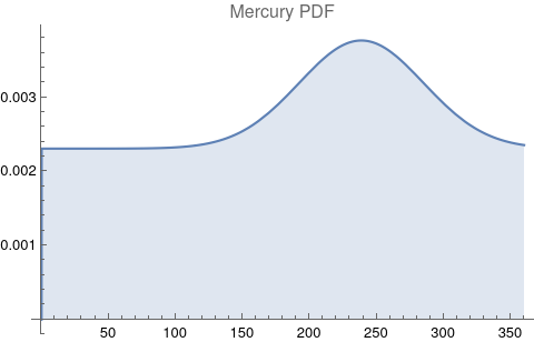
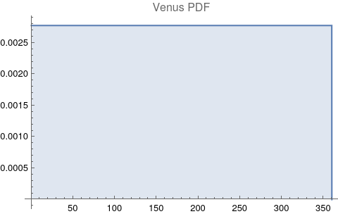
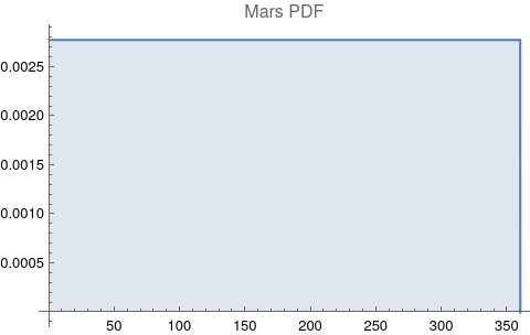
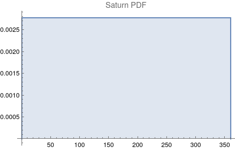
There are obvious spikes for some of these features. Perhaps the dramatic increase in the high 200's for the Sun degrees is most surprising. (There may be  more public news events in the northern hemisphere's late autumn and early winter when the Sun would be yearly at these degrees. For example, events around the USA Thanksgiving and Christmas holidays may register more as news-worthy.)

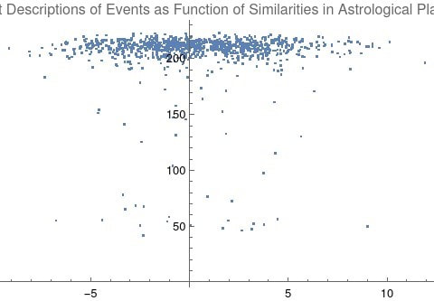
Comparing the 12-digit vectors for these zodiacal placements could be done by dot product too, but that would miss some very important features of astrology charts. We consider charts to be similar or conjunct when their degree differences, ie the results of their degrees’ subtractions, are either close to zero or close to 360 degrees or -360 degrees. Nicely enough, there is a trigonometric function that behaves exactly this way: the cosine. The simple plot of it follows, wherein you can see that the blue line has maxima at 0 degrees, 360 degrees, and -360 degrees.

Moreover there are other qualities of the cosine curve that preserve information from astrology. Oppositions at +/- 180 degrees are at -1, and +/-90 degree squares hold a value of zero. These parallel astrological interpretation wherein squares suggest no similarity, and oppositions do show similarity but of an opposite polarity as conjunctions. Degrees in between the extrema have cosine values that are appropriately in between as well.

Thus for each of the two events in an event pair, the twelve placements of the second one was subtracted from those of the first one. Applying cosine to each of the twelve differences and then doing a simple summation gives a single-number result that is a straightforward but robust metric for the 12-planet chart similarities.

Next is c., the assignment of detecting dependence. Note that this is different than correlation.

For example, a quartic is a function of the order of x raised to the fourth power. The resulting graph shows for each x one f(x), but it is not so that each f(x) only corresponds to one x. Parabolas, hyperbolas, and certain trigonometric functions such as cosine depicted above behave similarly.

Thus, one can say for these that f(x) is indeed a function of x, but not in a monotonic fashion. The idea of monotonic dependence is also known as correlation, but for these special non-monotonic functions, we need to consider tests for dependence and not correlation.

In short:

For dependency: determine that a variable has a value that depends on the value of another variable.

For correlation: the relationship between variables is linear and is considered as correlation. That is, as one similarity increases the other uniformly increases or decreases too.

This paper’s study answers a question not about correlation but about the more sophisticated situation of dependence.

To do the answering, I wanted a tool that can compute not just linear dependence (ie correlation) but also non-linear dependence.[10] Hoeffding’s D (for dependence) measure was selected.

Each Hoeffding D measure test was found to take about 16 seconds to compute for 100,000 event pairs, 22 minutes for 1,000,000 event pairs, and an unknown amount for the full event pairs that number over 25 million. The latter is unknown because the computation was aborted after six days. (The computer that was used is running Linux on an AMD 3950x CPU with 64 GB DDR4 RAM.)

Thus, a Monte Carlo approach was needed in order to estimate the upper-bound “p-hat” of the actual full p-value for independence. The approach consists of breaking up the problem into computing the p-value 100 different times for randomized sets that number 1 million pairs each.

The equation for this conservative upper bound is simply (r + 1)/(n + 1), where r is the number of runs that yield a test-statistic above that which is desired (here corresponding to a p-value of 0.05) and n is the number of different times the randomization is run (here equal to 100).[11]

All that is needed is r.

Results

The computations of n = 100 randomized runs resulted in an r value of 0.

Therefore, the p-value upper bound, also known as p-hat, is: (0 + 1)/(100 + 1) or 0.0099 < 0.01**.

In fact, for every one of the 100 runs of 1 million randomly selected pairs, the computed p-value was smaller than the smallest number the software can handle, 6^-1355718576299610, and for each of those 100 runs, a plot of event pair description similarities as a function of chart similarities was made.

The following is a movie of the 100 plots in sequence. Note the boundaries at x = +12, x = -12, y = 0, and y = around 250. These correspond to extremely similar charts, extremely dissimilar charts, dissimilar text descriptions, and similar text descriptions respectively.

To make it somewhat simpler to see the relationship, here is an example picture with just 1000 random pairs to show a general shape.

A likely dependent relationship between similarities in historical event text descriptions and similarities in historical event chart placements is thus established.

Example Case of Looking at a Specific Word, "Battle"

Calculating Hoeffding's dependence between each individual celestial feature and the 7153 distances to any given keyword is computationally tractable, even while computing across all keywords is not.

The following is a demonstration using the most frequent keyword in the event descriptions, "Battle".

To see how likely the resulting dependence measures are, a second, more specific Monte Carlo simulation of 10000 sets with 7153 randomized charts in each set was used to calculate p-values. The randomizations were distributed according to the PDFs of each celestial feature.

Celestial Feature                         Hoeffding's D                           Monte Carlo P-value
Sun                                                     0.015                                                << 0.00001          
Moon                                                  0.62                                                 << 0.00001 
Mercury                                             0.006                                               << 0.00001
Venus                                                 0.013                                                << 0.00001
Mars                                                   0.042                                               << 0.00001
Jupiter                                               0.15                                                  << 0.00001
Saturn                                                0.068                                              << 0.00001 
Neptune                                            0.47                                                << 0.00001
Uranus                                               0.01                                                  << 0.00001
Pluto                                                   0.13                                                  << 0.00001
North Lunar Node                          0.00                                                 0.47
South Lunar Node                          0.00                                                 0.26

Conclusions

In this paper, similarities in historical event descriptions are shown to be most likely a function of chart similarities with an estimated p-value upper limit for independence that is under 0.01.

A relationship between astrological chart similarities and event description similarities seems to exist. This relationship could well be employed to allow for event prediction based on a future day's projected geocentric astronomical placements.

Correspondence and not correlation was the focus as it appears in list plots that the state of textual similarities vary as a function of chart similarity.

There are some interesting connections to make from the plots of the two similarities. First, there is some imperfect symmetry across the y-axis, saying that very large positive-number chart similarities (indicating all close conjunctions) can behave somewhat like very large negative-number similarities.

The latter would occur when the twelve degree differences are all close to 180 degrees, ie when there are strong oppositions. That too is considered a strength between two charts, so this may be some empirical support for that belief in astrology.

In the example of pinning event description distance to the keyword "battle", the dependence measures of the nodes are not statistically significant, but everything else is. Moon and Neptune exhibit greatest dependence measures for "battle" which is astrologically surprising.

Some readers may be concerned that Neptune's dependence measure is high in that example, because it moves so slowly and hence may be associated with an era in time, ie an era with more battles.

That is where the second Monte Carlo significance comes in very handy. It tells us that, given the probability distribution for Neptune, the natural occurrence of such a high dependency measure is extremely unlikely.

As well, note that Uranus and Pluto do not show high dependence measures in this case, even though they move as slow or even slower than Neptune.

Moreover, the pre-eminence of the very quick-moving Moon and its uniform PDF negate the concern altogether.

Code is available, including for the generation of data.[12]

Works in Progress
To continue this study, work on the following has commenced.

1. Humanistic principal component analysis on the language of the astrological literature for each celestial feature ("Sun", "Moon", "Neptune", etc.) compared to to the most common words ("battle", "union", "premieres", "president", etc.) to see if it is related to the celestial feature Hoeffding measures of dependence.
2. Daily journal to track synchronicity between actual public events and those suggested by the events database for being similar to the chart of a day. (Early tests have shown not much success here. The event descriptions in the original database may not be rich enough to saturate all possible new events. I am working on some automated, quantitative approaches to demonstrate prediction confidence.)

References

1: Wolfram Research, EventData, 2012, https://reference.wolfram.com/language/ref/EventData.html

2: Wolfram Research, Wolfram Knowledgebase, 2022, https://www.wolfram.com/knowledgebase/

3: Wolfram Research, Frequently Asked Questions, 2022, https://www.wolframalpha.com/faqs/

4: Bengio Y., Ducharme R., Vincent P.,  and Jauvin C., A Neural Probabilistic Language Model, 2003, Journal of Machine Learning Research, 1137–1155,
https://www.jmlr.org/papers/volume3/bengio03a/bengio03a.pdf

5: Aylien.com, An overview of word embeddings and their connection to distributional semantic models, 2022, https://aylien.com/blog/overview-word-embeddings-history-word2vec-cbow-glove

6: Gärdenfors P., The Geometry of Meaning, 2017, MIT Press, https://mitpress.mit.edu/books/geometry-meaning

7: MIT Technology Review, King - Man + Woman = Queen: The Marvelous Mathematics of Computational Linguistics, 2015, https://www.technologyreview.com/2015/09/17/166211/king-man-woman-queen-the-marvelous-mathematics-of-computational-linguistics/

8: Wolfram Research, BERT Trained on BookCorpus and Wikipedia Data, 2022,
https://resources.wolframcloud.com/NeuralNetRepository/resources/BERT-Trained-on-BookCorpus-and-Wikipedia-Data/

9: Google Research Inc., Measuring Similarity from Embeddings, 2022,
https://developers.google.com/machine-learning/clustering/similarity/measuring-similarity

10: de Siqueira Santos S., Takahashi D., Nakata A., and Fujita A., A comparative study of statistical methods used to identify dependencies between gene expression signals, 2013, Briefings in Bioinformatics, 1-13, https://www.princeton.edu/~dtakahas/publications/Brief%20Bioinform-2013-de%20Siqueira%20Santos

11: North, B. V., Curtis, D., and Sham, P.C., A Note on the Calculation of Empirical P Values from Monte Carlo Procedures, 2002, American Journal of Human Genetics, 439 - 441, https://www.ncbi.nlm.nih.gov/pmc/articles/PMC379178/

12: Oshop R., Is Textual Similarity of Events Related to Event Chart Similarity?, 2022, www.wolframcloud.com/obj/renay.oshop/Published/Events%20comparisons%20published.nb

A basic video run-through of the above material follows.

Abstract

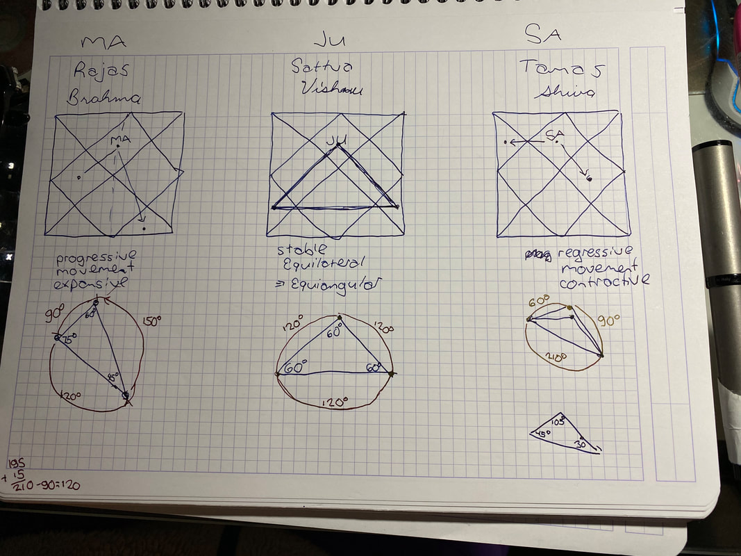
Contemporary astrologers are challenged like never before to make their work scientific. This is especially true for astrology researchers who are stewards of the keystone for legitimacy in astrology. Fortunately, current strides in artificial intelligence allow new avenues to data cultivation for the public and private astrology researcher. The author presents her freely available solution to the challenge, using in her explanation basic, intermediate, and advanced concepts.

The Challenge
​
Astrologers the world over from all times, whether Eastern, Western, Persian, Chinese, or Tibetan, face the same challenge. Event data of time, place, and date, including that of births, are mandatory for us to do our work.

Acquiring that data is more difficult than at first blush it may appear. For example, if one is interested in sports astrology and one wants to know the start of a basketball or cricket match from five years ago, how does one actually find that?

Perhaps there is an online news article from that time, but there are likely to be hidden problems. What I have found is that there is a wide variety among news publications as to how they treat such events. For example, BBC will include the time of the match in subsequent or preceding write-ups, while The New York Times will not.

Another part of the challenge is the language used in an article. For example, the article may say something like “the match happened last Sunday”. The New York Times often uses such an approach, begging the questions of which Sunday is that and what is its date. It may be obvious to the contemporaneous online reader but not to one years thereafter.

Then, there is a question of whether those articles are even archived and hence publicly accessible for some time later. Often, only the articles subsequent to an event are kept posted online and then only for a few years.

Finally, there is the strong possibility of an astrologer not knowing that the event exists in the first place. For example, let’s switch our focus to cyclone event data. There was a cyclone in the Spring of 2019 named Cyclone Ida.

There are hundreds of cyclones per year. (National Hurricane Center, 2019) Twenty years from now, will an astrologer who is interested in cyclones know to do an online search of contemporaneous literature for that particular cyclone? Will there still be material online for that cyclone?

Doing astrological research is difficult. For the cyclone researcher, he or she may need to pore over tens of thousands of webpages just to get that kernel of truth of when, where, and what time a batch of cyclone events occurred.

Reading that many documents takes time. Even if a list of ten thousand website URLs were presented instantly to the researcher, spending three minutes to scan each article would necessitate a solid 21 hours straight of such focused activity. That is not counting the search itself for the URLs or the recording of the results.

Given these daunting facts, there is no wonder as to why astrological research is relatively rare and often scanty or incompletely done. Science, by contrast, demands first and foremost the relative accuracy and completeness of data. This core difference between astrological research and conventional science represents the deepest chasm between the two world perspectives.

Bridging this chasm of data completeness would do the most to unify the work of all astrologers everywhere within the paradigm of science that could be said to define our current societies.

The Solution

A data challenge needs a data solution.

The Information Age in which we live deluges us with data. Fortunately, in these times, we are being presented with newly hatched tools to automate the search for and the processing and retaining of data in bulk. The newest and best methods use artificial intelligence (AI).

At this time, these AI tools are being used throughout every industry except astrology. These tools presently are also not for the mathematically faint of heart, so there is still a pretty steep learning curve for implementing them. Commercial industries find that the effort directed to the computational and mathematical gymnastics is more than worth it. The results are phenomenal, world-changing, and transforming to the industries even as the computer science in use is still relatively in its infancy.

What is needed is a means of using these tools to help the future astrology researcher who is within that exponentiating global data deluge to find and record the relevant data that was previously preserved as it happened.

Just as astrologers use books for transmission of knowledge, email for communicating with clients and each other, and software for chart generation, it is time for astrology to join the rest of professional society by investigating and employing the latest machine learning methods to generate artificial intelligence within astrology.

Event data generation is the first order of business for the personal or public research astrologer. Using artificial intelligence on global public information to cultivate event data should be the first order of business for a current computer scientist who wishes to help astrology.

Basic Ideas

There are a few steps to a computer-automated processing of current event data to help a future astrologer.

A computer program would be needed to 1. monitor daily current events as they are published in online articles. The computer program would then need to 2. linguistically digest the complex language of online news to find A. the nature of the event (for example, a new cyclone) and B. the date, time, and place of the event. After digestion, the computer program, at a minimum, would need to 3. preserve A. and B. for future use.

The basic triplicate of requirements of monitoring, digestion, and preservation of astrologically relevant data in a timely manner is in truth a cascade of separate algorithms, or sub-programs, each of which has only been developed recently, sometimes as recently as just a few months ago.

Monitoring can be done through a process called web scraping, wherein the texts of new articles are programmatically gleaned. However, of the millions of new articles that get published per day, which have data relevant to events of interest to the future astrologer? There is a computational cost to aggregating such monitored data. Even if the program takes but one second per article to seek out, acquire, and analyze for relevancy the text of the article, only 86400 such articles could be processed per day for this step alone. Thus, for current network, hardware, and software constraints, a necessary restriction in the numbers of internet sources and research topics is required.

Digestion is the most technically challenging part of the three-step process. The computer program would need to do nothing less than understand language itself. Take this sentence as an example: “Last Sunday night, three hours after kickoff, the Chicago Bears won the Super Bowl championship against the Denver Broncos.” The program would need to know that A. the article is about a match in American football and B. what was last Sunday’s date. The location and time of kickoff would, one hopes, similarly be determinable through other sentences of the article.

Digestion makes heavy use of something called natural language processing, a field of artificial intelligence that is still rapidly improving. The following two sections explore this step in some detail.

Finally, preservation of the data in a central, publicly accessible repository is the last, necessary step to the program. This is the easiest step of the three and typically just requires publishing the data file online.

Intermediate Ideas
​
Natural language processing (NLP) across different languages and across different subjects is a wide computer science field with many compartments. The main ones of relevance here are automatic summarization, natural language understanding, and question answering.

Automatic summarization is needed to determine whether an astrology research topic is indeed the topic of the article. Typically, this is done by condensing the article into a small summary and seeing if the topic is present therein. How does one determine the summary of an article? The non-trivial prospect of text extraction and synthesis based on statistical significance metrics and pattern-matching is a relatively straightforward type of summarization. These days, abstraction of language content is also often required as well. Machine learning based on linguistic feature extraction is at the core of this memory- and computation-heavy abstraction process. As a sub-field of NLP, automatic summarization benefits as being one of the longest studied topics of it. (Hahn & Mani, 2000)

Natural language understanding is the study of how to improve comprehension of text by a computer. It is a necessary middle step to answering questions from the text. The reader may be familiar with interfaces for language understanding from Siri, Bixby, or Alexa apps on their cell phones. Such commonness belies the extraordinary technical achievement that they represent. For example, one may say “The man started on a new novel,” and “The man started on a sandwich”. The formal structure is identical even though the meanings are wildly different.

Finally, question answering is critical to the astrologer’s needs. Even with the well-understood text of an article whose topic was deemed relevant, asking questions of the article is also non-trivial. Fortunately for astrologers, there are only three main questions. On what day did the event occur? At what time of day did the event occur? In what town did the event occur? However, the news article may be ambiguous on these matters or it may not include these details at all. For example, for a cyclone, what counts as the birth event? The initial early formation far off at sea? Landfall? Landfall only reaching a major population center? Such delicate domain-specific answering to a question is only lately, in the past few years or so, reaching maturity.

Advanced Ideas
​
The implementations of automatic summarization, natural language understanding, and question answering that are useful to know about for my project involve neural nets.

​Neural nets, a.k.a. artificial neural networks (ANN), are a way for the computer to solve problems of NLP that is lightly based on how biological animal brains work. Their loose depiction is as follows.

Visual examples of the special aspects as end points to triangles pictorially show the language that describes the planets Jupiter, Mars, and Saturn.

My derivation of the angle values:

[Edit: this study was subsequently repeated with NFL player data, and the same negative results held and in the same way.]

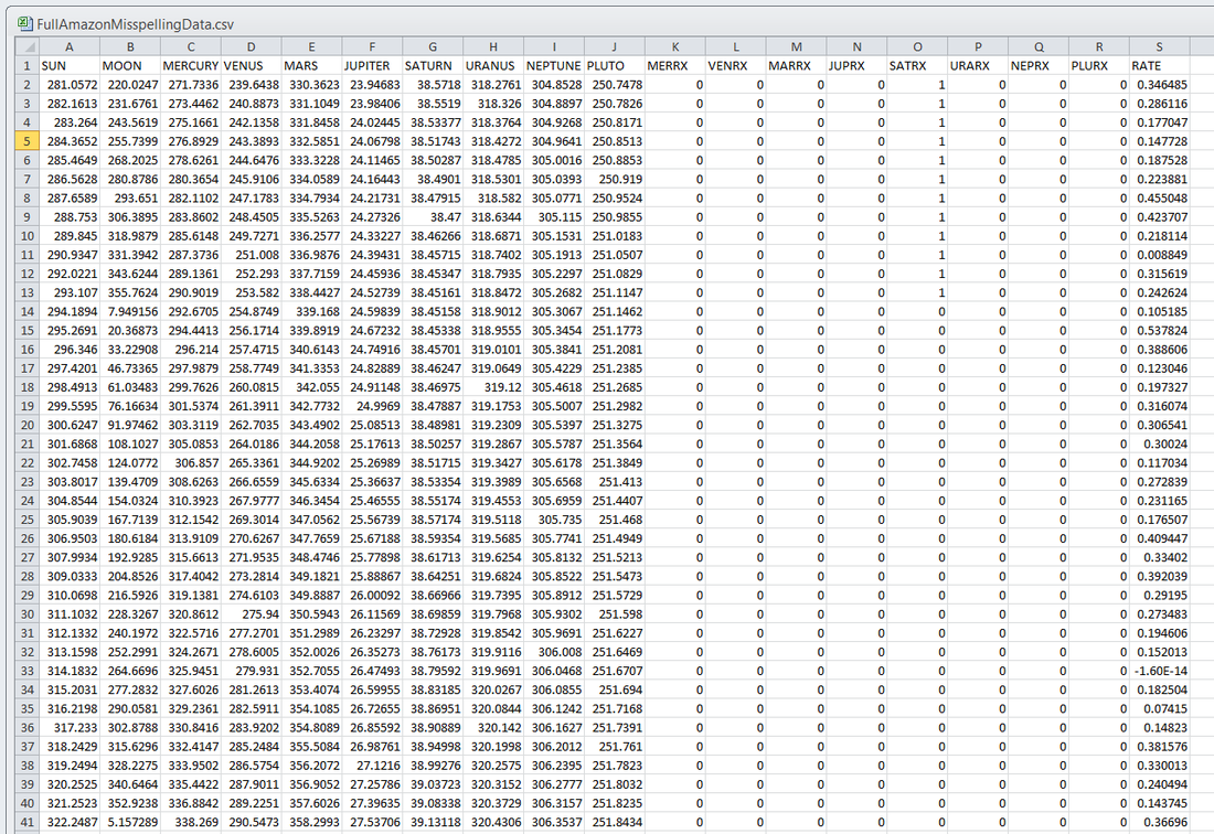
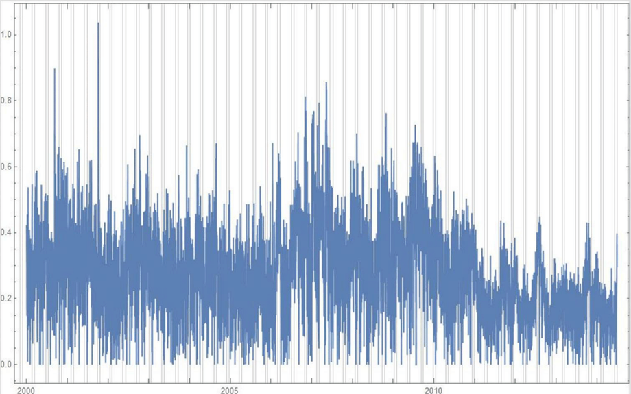
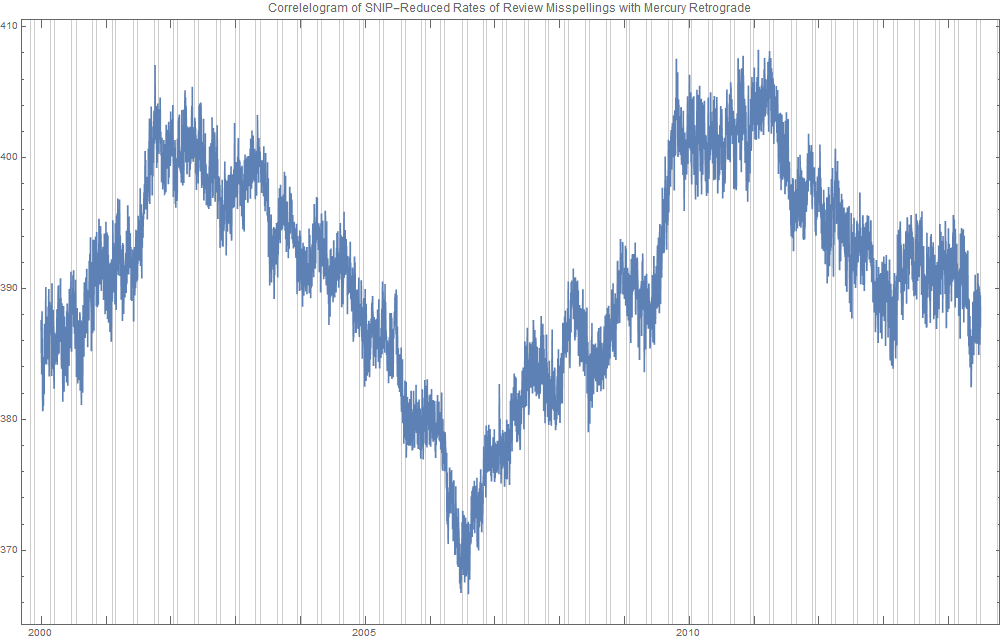
It was a topic of conversation: does body mass index (BMI) or even height or weight vary among the sun signs?

Ayurveda would say that they may vary by Ascendant, not particularly the sun sign, but getting good data on the Ascendant is a notable difficulty, because the Ascendant depends on the birth time of day.

Getting tens of thousands of charts with that level of precision is nearly unheard of.

A psychology prof from France named Michel Gauquelin compiled thousands of charts in the 1950's and 1960's that included birth time and hence Ascendant information. I am a little skeptical of the quality of these charts, as many are from the 1800's and more worringly, many use Local Mean Time, which if you back-engineer, describe the birth time as being at 10 am or 11 am on the dot.

So, I feel I can not use Gauquelin's data. I am always on the lookout, then, for credible birth or event data, scouring data science competition sites like Kaggle for the elusive ideal data set.  

I came across SoFIFA.com in that way. It gives very good data on the various thousands of professional male soccer players associated with FIFA, including their birth date and height and weight. Birth time and place are not given.

However, if I could just "scrape" that data, that would give me a way to test the conjecture that BMI or even height or weight may vary by sun sign. So, that is what I did. 

[Edit: The latest and greatest on this project, including source files, can be seen at ​the publication link here.]

I have posted a few times here about a rich dataset that I have.

Data were obtained from Stanford's SNAP data repository of Amazon.com reviews that gave daily misspelling rates; astronomical data were from Wolfram's Mathematica software and its astronomy resources.

Here is what the dataset looks like. Click on each picture to enlarge.

Each of the 5296 rows represents a sequential day in a 14.5 year span of Amazon review misspelling rates during Jan 1, 2000 to Jul 1, 2014.

Across the top are the labels. In each column is a simple, stable, linear function of the right ascension (i.e., the astrological Tropical degree) of the planet, moon, or star at midnight at the start of that day in London, UK. Retrogressions of the planets are also included.

The final column is the log of difference of the misspelling rate of the day from the 27-day SNIP baseline. (The Moon's right ascension completes its cycle every 27 and change days. That is the shortest cycle for any of the right ascensions.) Thus, it is the data over time minus its background noise. The following is a graph of this column's data over time.

SNIP stands for Sensitive Nonlinear Iterative Peak-clipping algorithm. This method preserves any cyclic patterns -- such as the planetary placements and retrogressions -- while discarding "background noise" in the data, which would tend to obfuscate the patterns. The SNIP method is not subjective. It comes out of processing signals within spectra and is unprejudiced. Note that the SNIP method comes from signal processing and tends to preserve cyclic behavior in spectra.

The apparent cyclicity hidden within this data is revealed via a correlelogram:

The thin bands represent the start and end of Mercury retrograde across 14.5 years with Mercury retrograde analysis being the original motivator for acquiring this data.

​​For today's study, the data for the first 80% of days were developed into a training group, and that of the subsequent 20% of days were isolated as a test group for prediction.

What was doing the training and testing? They were done entirely by an automated machine learning (AI) algorithm from BigML.com called DeepNet.  DeepNet* was applied to the training set of the first 80% of days. This DeepNet was then tested or evaluated on the last 20% of days. The DeepNet is a hands-off technique offered to anyone for free.

The chart below displays ridiculously good results as given in the usual AI industry way: the error rates for predictions for the 20% test group by DeepNet (in green) is dramatically smaller than other standard methods of prediction, in gray, which are based on the mean (average) rate of the training data or an approach assuming random chance. Moreover, the strong R-squared suggests good correlation of predicted misspelling rates to actual values only for the astronomical data of the DeepNet.

Astro-databank is the resource for researchers in astrology. It is a repository of birth information of many thousands of people and events and includes biographic data as well as the birth time, place, and date. Of high utility is the included Rodden Rating which tells us the accuracy of each chart.

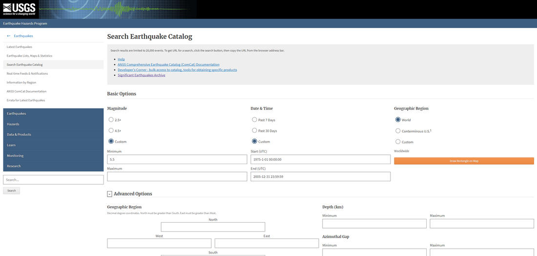
An AA rating is "Data as recorded by the family or state". The expectation of many researchers is that AA data is of the highest accuracy possible and can be used freely.  In the following, I show statistically that it is extremely unlikely that the AA rating charts altogether are accurate. I will be considering charts of people only and only those born at or after 1930.

From here on, I will try to state things as explicitly as possible.

The common assumption (the null hypothesis) is that AA rating charts are all of high accuracy and hence, taken altogether, exhibit behavior of high accuracy. My assertion (the alternate hypothesis) is that AA rating charts do not exhibit behavior of accurate birth data.

One behavior of accurate birth data is that the minute of birth is evenly distributed. That is to say, a birth time of 8 minutes after the hour is not expected to happen much more or less than a birth time of 9 minutes after the hour, for example. 

The following is a simulation of a uniform distribution so that you you know what its plot looks like.

When it comes to modeling real-life phenomena for astrological research, earthquakes are one of the most widely studied.

And why not? After all, the exact time, place, and day are known as well as the strength of the effect (in magnitude).

However, a mapping of earthquake strength to solar system events has proven to be elusive, not to be dramatic, but until now.

Inspired by this Kaggle post, I decided to try my hand at this perhaps age-old problem, and I found that yes, earthquake magnitude correlates with the moon phase at the time of the event. (Moon phase has been looked at quite often but not with the model I will present today.)

First off, I went to https://earthquake.usgs.gov for the earthquake data. (Thanks to Joe Ritrovato for the link.)

​I wanted to look particularly at all earthquakes of any depth between Jan 1, 1975 and Jan 1, 2005. Those years were chosen, because a uniform seismograph was finally used through out the world by the mid-1970's, and hydraulic fracturing with its associated quakes was not yet in widespread practice. The search was further restricted to earthquakes of magnitude greater than 5.5, following this system of what counts as a serious earthquake. (Some lower limit to the magnitudes was necessitated by the search limit on the USGS site.)

Here is what my search looked like (be sure to also choose earthquakes only below the fold):

And here is what you will see if you press enter: