1. Introduction
“Mercury retrograde” is, in my culture, a time of great concern.
It is believed by many that the apparent astronomical retrogression affects human communication, travel, use of electronics, and thinking, among other broadly related things.
To test the general thesis of an effect on communications during Mercury retrograde, I looked at a randomized 5% of a collection of 69,242,585 Amazon reviews posted between Jan 1, 2009 and July 23, 2014. (Amazon.com: Online Shopping for Electronics, Apparel, Computers, Books, DVDs & more n.d.)
I counted the number of words per entry that are not in a computerized dictionary, while discounting digits, internet links, emoji, words with three or fewer characters. Non-English entries were also discarded.
As well, not considered were context mistakes (such as there/their/they’re), grammar, punctuation, or capitalization errors. I wanted to simply approach comparing occurrences of larger non-dictionary words in Mercury retrograde seasons versus non-Mercury retrograde seasons.
2. Materials
The source of the millions of Amazon reviews is a big data repository held by Stanford University. (Jure Leskovec and Andrej Krevl 2014) The Amazon data in particular is managed by Julian McAuley who kindly made it available to me for research purposes. (J. McAuley 2015)
I chose an “aggressively deduplicated” version of the dataset that has no duplicated entries whatsoever. This data represents all 82.84 million Amazon product reviews with metadata to the date of July 23, 2014.
3. Methods
The software Mathematica was used to implement standard data science and signal processing techniques. (Wolfram Research, Inc. 2015) The algorithms are publicly available. (Oshop, Zenodo 2015)
First, the data was scrubbed of 16.04% of its 82,469,759 entries, as these proved to be nonstandard JSON (the main format of the database) and could not be evaluated by Mathematica itself. Since automating analysis of such a large dataset would be a primary key to any success, I was comfortable with the percentage lost. However, whether there is some important unifying theme to the lost entries, such as Amazon product department, time of submission, etc. is not known by me. Using such large datasets (here, 57 GB uncompressed) is still something of an art form, especially for an older dataset, even by the best operators of the best technologies.
Thus, a table of 69,242,585 lines was built with two entries per line: the time of the original entry in Unix format and the review text, including edits. No record exists in this database of the timing of the edits to the review.
Next, I programmed an evaluation that used a random number generator and the built-in dictionary to analyze a randomized choice of 5% of all entries. (DictionaryLookup Source Information—Wolfram Language Documentation n.d.)
Each entry’s review was split into textual word substrings. To find emojis and links, the word strings had to be analyzed character by character.
After that, if the dictionary found no match to the word string, it was counted as a “misspelling” in that entry. A sum of these entry misspellings was divided by the number of total textual words in the entry and the result was recorded along with the day of the original submission.
Even with a randomized sampling of only 5%, running this program took about 31 hours on my desktop computer, at a rate of analysis on the order of 1,000 entries per second.
Note that this technique would consider an unusual brand name of a product, for example, as a misspelling which would be introduced as a kind of noise to any more general trend.
The resulting entries were grouped by date. A day’s group mean was recorded with that date and retained. These values for all dates in between January 1, 2009 and July 23, 2014, GMT, were built into a time series.
A mean filter was applied to the time series, and the results were plotted along with it.
The difference between the actual mean value for the day and the trend from the filter was found though subtraction and plotted.
A variety of periodicities emerged. That variety was analyzed through a discrete Fourier transform. The main structure, coming from the contribution of the highest two values, was graphed and found to correspond well to the regular periodicity of Mercury retrograde.
In the following pictures, the thin vertical bands mark the actual demarcations of Mercury retrograde, GMT, in that time frame.
4. Results
A. Movement of Daily Averages
The blue line describes the up and down movement of actual daily averages. The lighter gold line depicts the general trend. This general trend was obtained by a mean filter on the blue data.
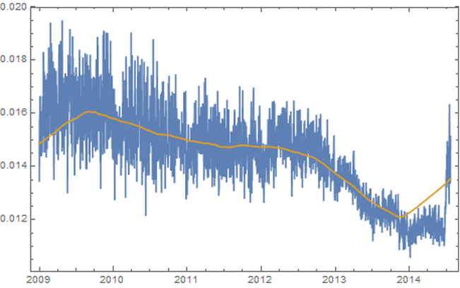
Because of the nature of a mean filter, the right and left end regions are not as accurate, which you can see in the above graph. They were excised from consideration. Accordingly, the following analyses include only date values between July 1, 2009 and July 1, 2013, still a rather long time length of four years.
B. Differences of the Daily Averages from the General Trend
The trend filter value (gold in Figure 1) was subtracted from mean filter value for each day (blue) and the result was plotted.
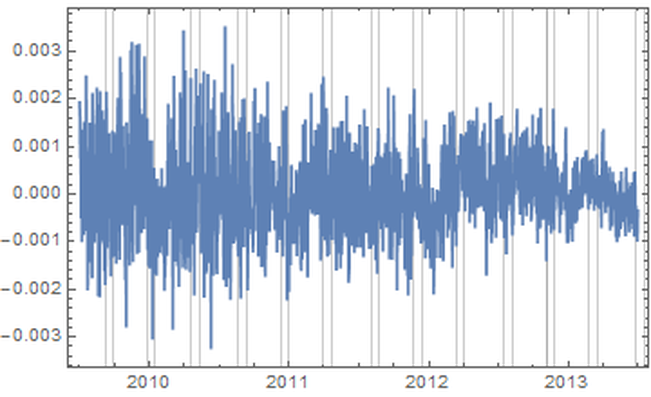
These differences between actual daily value and the general trend were subjected to discrete Fourier transformation. The spectrograph is below.
1. Plot of Discrete Fourier Transform of Differences
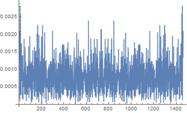
The fundamental first line is the highest at 9 along the horizontal axis, and the second major peak is at 13. With these numbers, along with their heights, we can construct the major course of the data, i.e., the wave that contributes the very most to the rise and fall of daily misspelling rates in Amazon reviews.
2. Construction of the Sum of Fundamental and First Major Harmonic
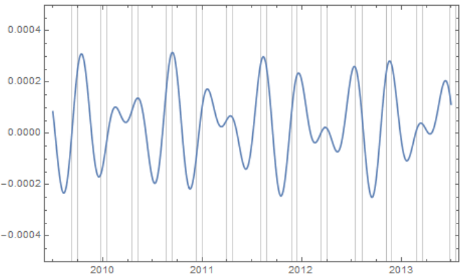
As you can see, before each non-Mercury retrograde time marks the local and global minima of non-dictionary word use rate with a rise to the local and global maxima all occurring in Mercury retrograde.
[Edit: If you like even cleaner data and would like to see an even more perfect graph, see this more recent post, where I improve the evaluation algorithm slightly but reasonably which was enough to change the fundamental to exactly Mercury retrograde.]
5. Discussion
Looking much like software’s graph of an audio clip of the human voice, Figure 2 might at first seem fascinating but opaque to easy interpretation.
In the case of the audio’s graph, the sound it represents is all in there, but how do you get from the visual picture back to the sound again? After all, recording, compressing, transmitting, and recreation of audio all happen from such software.
There has to be a mathematical way, and there is. One of the major tools of science of the last one hundred years is the Fourier transform.
Think of someone playing a pure middle C note on a perfect piano. The Fourier transform would break down that note to a graph much like Figure 3, only there would just be a single line on the left (with its mirror on the right), also called the fundamental: the one matching the frequency of middle C.
In Nature, things tend to be more complicated. An actual piano would likely have rough, very minor sub-harmonics that build on and modify the major one. The major one would still have the exact shape of the sinusoidal wave of perfect middle C, but these rough minor frequencies would adjust that first dominant curve into a final wave form that is more complicated than, but resembling, a pure C note.
This set of more minor notes would also appear on the Fourier transform plot, but as shorter lines and at placements along the horizontal axis that correspond to each of their frequencies. The heights give their order of modification of the first, fundamental note. Typically, the whole wave can be summarized in just a few lines. That is how compression and removal of noise in sound happens.
Returning to the sound of the human voice, the complex stacking of a rich variety of sub-harmonics could still be teased apart by the wonder of the Fourier transform, but into dozens of lines.
Similarly, looking at the wave form of Figure 3, there are dominant “notes” that can be pulled out, and the most fundamental, dominant one of all, the one that all others modify, is at a frequency band of occurring approximately once every 142 to 162 days, with a phase shift for the time window of -2.90338. This is the highest band at position 9. The major, first harmonic appears next in height (and strength of effect) at the 13 position which represents a frequency band of occurring approximately once every 111 to 115 days, with a phase shift for the time window of 1.05873, the very frequency and phase shift of Mercury retrograde itself in the time period being considered.
Adding the fundamental and first harmonic together, we obtain a wave, and as seen in its graph in Figure 4, the lowest troughs of the wave all happen in between the periods of time also known as Mercury retrograde with the highest peaks all in Mercury Retrograde.
6. Conclusions
The results of this study are still a ways away from proving that Mercury retrograde causes spelling errors, although, with this study, an important first step has been established. Herein is just proof that the period also known as Mercury retrograde is a uniform time of maximum periodic contribution to non-dictionary word use in the dataset, an increase that can be as high as 2.19%.
If this small, but significant, error rate boost in a single act would hold across a series of them, then compounded across the thousands of small things that we do each each day, it would make one virtually sure to make a big mistake (one that is built from the small steps) during the 21 - 23 days of a Mercury retrograde period.
A remarkable side note is that the two percent, statistically significant increase was the same found during Mercury retrograde for a completely unrelated database’s non-dictionary use rate during a completely different period. (Oshop, Across Millions of Entries, Reddit is More Likely to Show Misspellings During Mercury Retrograde in May 2015, 2015)
There may still be some unknown market or cultural factor that has exactly the same periodicity and starting point as Mercury retrograde. If so, that would still suggest a tendency, actually an absolute correlation, to increased use of non-dictionary words during Mercury retrograde seasons. People who believe in some increased danger of error during that time would still be right.
The poetic turn of phrase of the harmonics of the spheres may be no mere metaphor.
Works Cited
- Amazon.com: Online Shopping for Electronics, Apparel, Computers, Books, DVDs & more. n.d. amazon.com (accessed 10 24, 2015).
- “DictionaryLookup Source Information—Wolfram Language Documentation.” Wolfram Language & System Documentation Center. n.d. reference.wolfram.com (accessed 10 24, 2015).
- Discrete Fourier Transforms—Wolfram Language Documentation. n.d. reference.wolfram.com (accessed 10 25, 2015).
- J. McAuley, R. Pandey, J. Leskovec. “Inferring networks of substitutable and complementary products.” Knowledge Discovery and Data Mining, 2015.
- Jure Leskovec and Andrej Krevl. SNAP Datasets: Stanford Large Network Dataset Collection. June 2014. snap.stanford.edu/data (accessed 10 24, 2015).
- Oshop, Renay. Across Millions of Entries, Reddit is More Likely to Show Misspellings During Mercury Retrograde in May 2015. 10 10, 2015. Read on this site (accessed 11 2, 2015).
- Oshop, Renay. Non-Dictionary Words Occur More Often in Amazon Reviews During Mercury Retrograde. Zenodo, 2015. DOI: 10.5281/zenodo.32847
- Wolfram Research, Inc. Mathematica. Version 10.2. Champaign, IL: Wolfram Research, Inc., 2015.
I wrote this in November 2015. It is the most careful thing in this sequence — numbered sections, citations, deposited code — and I have left every word of it above as it was. Being careful turns out not to be the same as being right.
The design faults this shares with the two Reddit pieces are set out at length on the earlier article and I will not repeat them here. These are the faults belonging to this one.
My strongest signal is not Mercury
Read my own Results again. The fundamental — the most fundamental, dominant one of all, the one that all others modify
— sits at position 9, a cycle of 142 to 162 days. That is not Mercury retrograde. Mercury is at 13. So the loudest rhythm in my own data is something I never identified, never chased, and mentioned only in passing on the way to the peak I was hoping for. My headline rests on the runner-up.
And 13 is not a harmonic of 9
I called 13 the first major harmonic
and reached for a piano to explain what that meant. But harmonics are integer multiples of a fundamental: the harmonics of 9 are 18, 27, 36. Thirteen is not among them. Nine and thirteen are simply the two tallest spikes in a noisy spectrum, with no musical relationship to one another whatsoever. Fundamental chord with first major harmonic
names a structure that is not there, and the metaphor did a great deal of work I had not earned. On a true middle C, as I wrote myself, the transform gives you a single line. Look at my Figure 3. It gives a forest.
Nothing in that forest is taller than noise makes
Here is the test I never ran, and it is the one that decides the article. Take a series of pure noise with the same day-to-day stickiness as mine — no Mercury in it, no signal of any kind, nothing. Run it through exactly my pipeline: mean filter, subtract the trend, transform the difference. It yields a tallest peak every single time, and that peak stands about three times above the middle of its spectrum. Now look at Figure 3. My tallest spike is about three times the height of the forest around it. That is precisely what nothing looks like. I never asked how tall a peak must be before it is allowed to mean something. The answer is: taller than mine.
Figure 4 is not evidence. It is my filter.
I kept two frequencies out of roughly seven hundred and threw the rest away, then presented what was left as the major course of the data
. Of course it is smooth. Discard 99.7 percent of a spectrum and whatever survives is a clean wave — do it to noise and you get a clean wave too. Worse, the wave I kept rises and falls about thirteen times across four years, and Mercury goes retrograde about thirteen times across four years. Two things that oscillate thirteen times in the same window will appear to keep time with one another whatever their phase. The eye finishes the job, and I invited it to: as you can see, before each non-Mercury retrograde time marks the local and global minima...
Looking is not a test.
Note the scale, too. The wave in Figure 4 swings by about ±0.0003. The daily movement it claims to describe, in Figure 2, swings by about ±0.0015. My major course of the data
is a small fraction of the thing it is named after.
Then I deleted words until Mercury won
The bracket I added later says it outright, and I will let it testify against me. I improved the algorithm slightly but reasonably which was enough to change the fundamental to exactly Mercury retrograde.
I dropped dvds
, DVDs
, apps
and Apps
; the peak at 9 shrank; 13 rose into its place. I announced that as the data coming clean. Read it the other way round: I adjusted the analysis until the frequency I wanted finished first, and then wrote a second post celebrating the improvement. I did not do this dishonestly, and that is the trouble. I did it because I already knew what I was looking for — which means I would not have noticed myself doing it.
Two more things I should not have waved through
I discarded 16.04 percent of the entries as unparseable and wrote that whether there is some important unifying theme to the lost entries... is not known by me.
That is a sixth of the database gone for reasons I could not characterize, and I let it by with a shrug because the alternative was tedious. And by my own admission an unusual brand name counts as a misspelling — but new products launch on a seasonal calendar, so my brand-name noise carries a rhythm of its own. A cycle of about 150 days is a good deal closer to a shopping season than to a planet, and I never once asked what my fundamental at 9 actually was.
The corroboration that was not one
In my Conclusions I call it a remarkable side note
that the same two percent turned up in a completely unrelated database
. The databases were unrelated. The analyst was not. Both studies were built by me, with my method, my exclusions and my expectations, within a month of one another. Two measurements taken by the same hand agreeing is not replication; it is consistency, which is precisely what a procedure that leans one way will give you twice. I offered my own repetition as though it were somebody else's confirmation.
The test, run at last
I have now run the test properly, on my own data file, and I am going to set the result down plainly because it is not what I wanted.
First, honestly, about what the file is. The daily averages plotted in Figure 1 above are gone — I have the recipe again and not the ingredients. What survives is fullamazonmisspellingdata.csv: 5,295 consecutive days from 2 January 2000 to 1 July 2014, each row carrying the longitudes of the planets, a retrograde flag for each of them, and a misspelling rate. Its rate averages about 0.24 where Figure 1 runs near 0.016, so this is a differently-built series and not the one behind this article. It is nonetheless my data, on my hypothesis, across 49 Mercury retrogrades. The file is here; judge it yourself.
One thing before anything else: fifteen cells in that file are not numbers at all. They read Mod[QuantityMagnitude[UnitConvert[Missing["RetrievalFailure"], "Degrees"]], 360] — Mathematica's ephemeris lookup failed on a few days for Uranus, Neptune and Pluto and wrote its own error message into my data where a longitude should be. I never noticed. The rate and the retrograde flags are clean, so nothing below depends on it, but I had published a file with my software's failures sitting inside it for eleven years.
The replication. Put that series through the method of this article — mean filter, subtract the trend, transform the difference — and my peaks come back. With a filter width of 121 days the tallest bands land at 13, 8 and 9. That is close to the 9 and 13 I reported in 2015, and for a moment I was pleased. Then I asked the question I had never asked: how tall does a peak have to be? I built surrogate series carrying my own spectrum but with the phases scrambled, so that any real timing is destroyed and only the shape of the noise survives, and pushed those through the same pipeline. My tallest peak stands 3.46 times the middle of its spectrum. The scrambled series average 3.33 and reach 4.05 one time in twenty. My peak's p-value is 0.383. The band at 13 — Mercury's — comes in at 0.148. So the pattern replicates and the meaning does not. The peaks are really there in the data. They are simply the size that nothing is.
And then the control I should have run in 2015. My file does not only flag Mercury. It flags the retrogrades of Venus, Mars, Jupiter, Saturn, Uranus, Neptune and Pluto as well, and I never once looked at them. So I tested all eight, identically: slide each planet's flag to every possible position and ask whether its true alignment stands out.
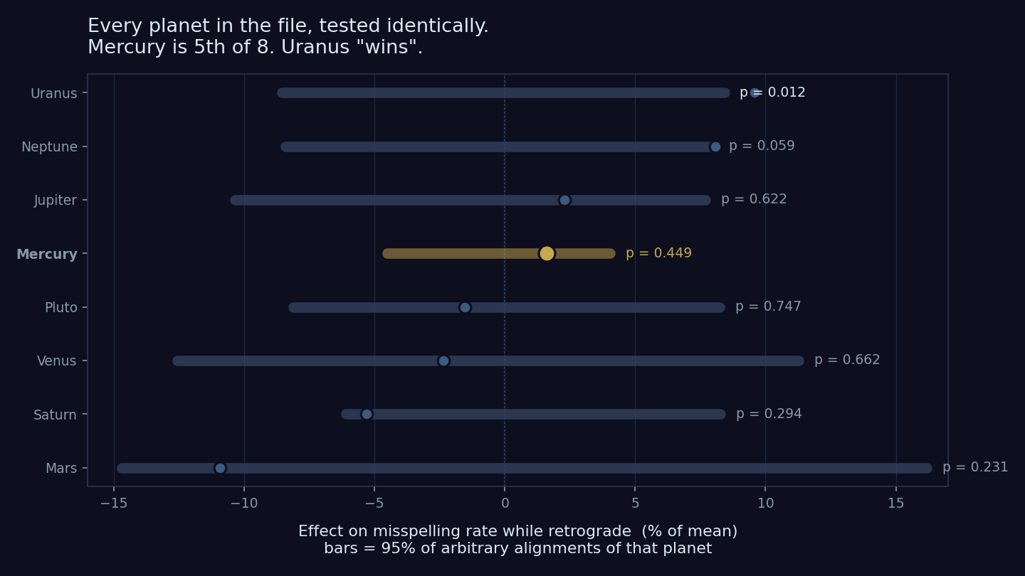
Mercury comes fifth of eight. Its 1.62 percent sits quietly inside the range that arbitrary alignments produce: p = 0.449. Mars shows an effect nearly seven times the size of Mercury's, at −10.94 percent, and it is not significant either. And the planet that does clear the usual bar is Uranus, at +9.59 percent, p = 0.012 — with Neptune close behind at 0.059.
I want to be careful here, because it would be easy to score a cheap point off myself. Uranus is not a discovery. Test eight planets at the five percent level and there is about a one-in-three chance that at least one clears it by luck alone; a correction for having taken eight bites gives Uranus a threshold of 0.00625, which it misses. Uranus is exactly what a false positive looks like — and that is the whole lesson, because it is also exactly what my Mercury result looked like to me in 2015. The difference is that I went looking for Mercury and would never have gone looking for Uranus. Had my culture worried about Uranus retrograde instead, this file would have handed me a publishable finding, and I would have written it up with the same care and the same conviction, and been just as wrong.
A predictor, and what it actually learned
The file carries the longitude of every body for all 5,295 days, so one more question is available now that I could not have asked in 2015: never mind explaining the past — can the sky predict the misspelling rate? I built a model and gave it everything. All ten longitudes, encoded as angles so that 359° sits beside 1°, plus all eight retrograde flags. Twenty-eight features.
Then the only part that matters: how to hold data back. My first instinct was to train on 2000–2010 and predict 2011–2014, and the model failed spectacularly — but that test was unfair, and not in my favour. The misspelling rate falls by half across this file, and the likeliest reason has nothing to do with the heavens: browser spellcheck and phone autocorrect arrived and got good during exactly these years. Asking a model to leap that gap is asking it to predict a technology, not a planet. So I hold out the middle instead — 2008 to 2011, training on the years either side — and also a plain random sample across the whole span. Neither asks the model to guess at a future it has no business knowing.
| What the model is given, and what it is asked for | Random sample | Held-out 2008–11 |
|---|---|---|
| All 10 planets + 8 flags → misspelling rate | 0.1759 | 0.1650 |
| All 10 planets + 8 flags → the calendar date | 1.0000 | 0.9999 |
| Fast bodies only (Sun…Mars) → misspelling rate | 0.0240 | −0.0438 |
| Mercury alone → misspelling rate | 0.0108 | 0.0113 |
| Day of the week alone → misspelling rate | −0.0005 | −0.0015 |
The first row looks like a discovery. Seventeen percent of the variance in human misspelling, out of sample, from the positions of the planets — and it holds up whether I sample at random or hold out three whole years in the middle. In 2015 I would have had that written up inside a fortnight.
The second row is why it is not a discovery. I asked the same twenty-eight features to predict, instead of the misspelling rate, what day it was. R² = 0.9999. The sky reconstructs the calendar essentially perfectly, because that is what a sky does. Saturn, Neptune and Pluto do not complete a single circuit of the zodiac in fourteen and a half years — their longitudes never wrap even once in my file, and each tracks the date at a correlation near 0.99. They are not planetary influences on anything. They are a clock in fancy dress, and I handed my model a clock and then congratulated it for knowing the time.
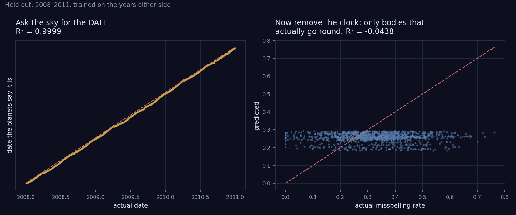
Everything that first row knows about misspelling, it knows by knowing the date — and the date is worth knowing, because the rate slides downward all through my file as spellcheck spreads. The planets are just the route by which the calendar got in.
So take the clock away. Keep only the bodies that genuinely go round and round within my window — the Sun, the Moon, Mercury, Venus, Mars, all of which wrap many times over and so cannot stand in for the year — and drop the slow outer planets whose position is merely a date stamp. That is the honest question: does the cyclical sky, the part that actually recurs, know anything about how people spell?
It does not. R² = 0.024 on a random sample and −0.044 on the held-out middle years — which is to say nothing, and then slightly less than nothing. The right-hand panel above is that result: a flat smear. Whatever the rate is doing on a given day, the recurring sky has no opinion about it. Mercury alone manages 0.011, and even that little is the season talking, since Mercury never strays more than 27.3° from the Sun and its longitude correlates with the Sun's at 0.96. A Mercury
feature is a time of year feature wearing my planet's name.
I should be straight about which way this cuts, because I have been wrong once already in this postscript. The seventeen percent is real. A model given the planets really does track my data better than a model given nothing. But it tracks it the way a stopped clock's neighbour does — by reading the date off Pluto and remembering what Amazon reviews looked like that year. Strip out the date and the sky is empty. I spent 2015 marvelling that the heavens knew something about my data. They did. They knew what year it was.
Where that leaves me. I did this one properly and it came out the same, and that is the part worth sitting with. The citations, the deposited notebook, the numbered sections, thirty-one hours of my desktop grinding through sixty-nine million reviews — none of it saved me, because the fault was never in the execution. It was in never once asking what my data would look like if there were nothing in it. I had a spectrum that noise could have produced, a fundamental that was not the planet, a harmonic that was not a harmonic, and a picture built from two percent of what I knew. I called it a result. And when I finally ran the controls, my own file preferred Uranus, and my own model turned out to be reading a calendar. I wrote in 2015 that the harmonics of the spheres may be no mere metaphor. On this evidence they are a metaphor — and I would rather be the one to say so. The most careful piece in this sequence is the most misleading of them, precisely because the care is so visible and the missing question is not.